Integration Milestone Pf
This notebooks executes IMpf. Details about the milestone, execution and verification can be found in tstn-031.
Keep in mind that in this execution we are more interested in the control flow, making sure that the expected data is published by the CSC, rather than validating that the data makes sense. Analysing the data and verifying that it has the expected values is a somewhat more involved tasks and requires some knowledge of the details of the wavefront estimatimation pipeline and the optical feedback control algorithm. These will, most likely, be part of a separate activity.
import os
import copy
import yaml
import asyncio
import logging

import numpy as np
import matplotlib.pyplot as plt

from lsst.ts import salobj
from lsst.ts import idl
from lsst.ts import utils

from lsst.ts.observatory.control.maintel import MTCS, ComCam
from lsst.ts.observatory.control.utils.enums import RotType
lsst.ts.utils.tai INFO: Update leap second table
lsst.ts.utils.tai INFO: current_tai uses the system TAI clock
Basic definitions
This section defines the basic SAL communication and control classes that are used to drive the system.
STD_TIMEOUT=5
domain = salobj.Domain()
mtcs = MTCS(domain)
mtcs.set_rem_loglevel(logging.ERROR+1)
MTHexapod INFO: Read historical data in 0.04 sec
MTHexapod INFO: Read historical data in 0.04 sec
await mtcs.start_task
[None, None, None, None, None, None, None, None, None, None]
Setting up the system
In order to execute the IM we need to make sure the MTCS components are in ENABLED state, that M1M3 is raised and the force balance system is enabled in both M1M3 and M2. We also want to enable the compensation mode on both the Camera and M2 Hexapods, though this is not strickly required.
Enable all MTCS components
The following cell will make sure all MTCS components are in enabled state.
await mtcs.enable(settings=dict(mtm1m3="Default"))
MTCS INFO: Enabling all components
MTCS INFO: All components in <State.ENABLED: 2>.
Setup M1M3
The following cells will raise M1M3, switch on the force balance system and reset the forces. We make sure to reset the forces so that we know the system is in the standard state, without any additional forces applied by previous users.
await mtcs.raise_m1m3()
MTCS INFO: M1M3 current detailed state {<DetailedState.ACTIVEENGINEERING: 11>, <DetailedState.ACTIVE: 7>}. Nothing to do.
await mtcs.enable_m1m3_balance_system()
MTCS WARNING: Hardpoint corrections already enabled. Nothing to do.
await mtcs.reset_m1m3_forces()
Setup M2
The following cells will enabled the force balance system and reset the forces on M2. As with M1M3, we reset the forces to make sure the sustem is in the standard state, without any additional forces applied by previous users.
await mtcs.enable_m2_balance_system()
MTCS INFO: M2 force balance system already enabled. Nothing to do.
await mtcs.reset_m2_forces()
Setup Camera Hexapod
The following cells will enable compensation mode and reset the position of the Camera Hexapod.
await mtcs.enable_compensation_mode("mthexapod_1")
MTCS WARNING: Compensation mode for mthexapod_1 already True. Nothing to do.
await mtcs.reset_camera_hexapod_position()
MTCS INFO: Camera Hexapod compensation mode enabled. Move will offset with respect to LUT.
MTCS INFO: Camera Hexapod in position: False.
MTCS INFO: Camera Hexapod in position: True.
Setup M2 Hexapod
The following cells will enable compensation mode and reset the position of the M2 Hexapod.
await mtcs.enable_compensation_mode("mthexapod_2")
MTCS WARNING: Compensation mode for mthexapod_2 already True. Nothing to do.
await mtcs.reset_m2_hexapod_position()
MTCS INFO: M2 Hexapod compensation mode enabled. Move will offset with respect to LUT.
MTCS INFO: M2 Hexapod in position: False.
MTCS INFO: M2 Hexapod in position: True.
Setup MTAOS
To execute IMpf we need to load a special configuration on the MTAOS. This configuration will make sure the MTAOS is reading data from a butler instance that was previously prepared for the test, and will also make sure the MTAOS is configured for processing LSSTCam Corner Wavefront Sensor data.
We start the process by first sending the MTAOS to STANDBY then sending it back to ENABLED with the required configuration.
await mtcs.set_state(
    state=salobj.State.STANDBY,
    components=["mtaos"]
)
MTCS INFO: All components in <State.STANDBY: 5>.
await mtcs.set_state(
    state=salobj.State.ENABLED,
    settings=dict(mtaos="impf"),
    components=["mtaos"]
)
MTCS INFO: All components in <State.ENABLED: 2>.
We also set the CSC log level to DEBUG, so we can debug the wep processing steps.
await mtcs.rem.mtaos.cmd_setLogLevel.set_start(
    level=logging.DEBUG,
    timeout=5
)
<ddsutil.MTAOS_ackcmd_fd03e870 at 0x7fce8479b220>
Processing data with runWEP command
Processing data throught the MTAOS requires sending the command
runWEP to the component. The command accepts a yaml configuration
that is used to control how the wep pipeline executes. We also need to
provide the id of the visit to process.
For reference we will also estimate the time it takes for the command to complete, though it is worth mentioning that this information is also published by the CSC.
wep_config = yaml.safe_dump(
    {
                "tasks": {
                    "generateDonutCatalogWcsTask": {
                        "config": {
                              "connections.refCatalogs": 'ps1_pv3_3pi_20170110',
                              "filterName": 'g',
                              "referenceSelector.doMagLimit": True,
                              "referenceSelector.magLimit.maximum": 15.90,
                              "referenceSelector.magLimit.minimum": 8.74,
                              "referenceSelector.magLimit.fluxField": 'g_flux',
                              "doDonutSelection": True,
                              "donutSelector.fluxField": 'g_flux',
                        }
                    }
                }
            }
)
Before executing the command, let’s clear the events we will want to check afterwards. This is mostly to make sure there are no previous events in the queue that could affect the verification process afterward.
mtcs.rem.mtaos.evt_wavefrontError.flush()
mtcs.rem.mtaos.evt_wepDuration.flush()
start_time = utils.current_tai()
await mtcs.rem.mtaos.cmd_runWEP.set_start(
    visitId=4021123110021,
    config=wep_config,
)
end_time = utils.current_tai()
print(f"Execution took {end_time-start_time}s")
Execution took 289.32793498039246s
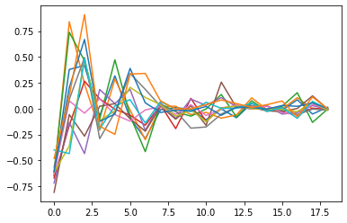
Verify output
To verify the execution we will check the wepDuration and
wavefrontError. The first one contains the measured execution time
done by the CSC whereas the second contains a set events with the result
of the wavefront estimation pipeline.
The CSC publishes one sample of wavefrontError for each pair of
donuts processed, so there are a number of events published.
print(await mtcs.rem.mtaos.evt_wepDuration.next(flush=False, timeout=STD_TIMEOUT))
private_revCode: 20fbb051, private_sndStamp: 1646437733.040275, private_rcvStamp: 1646437733.04058, private_seqNum: 7, private_identity: MTAOS, private_origin: 38497, calcTime: 290.7162170410156, priority: 0
The next cell will loop over the events and save the results to a list so we can plot them afterwards.
wavefront_errors = []

while True:
    try:
        wfe = await mtcs.rem.mtaos.evt_wavefrontError.next(flush=False, timeout=1)
        wavefront_errors.append(wfe)
    except Exception:
        break
for wfe in wavefront_errors:
    plt.plot(wfe.annularZernikeCoeff)
print(wavefront_errors[0])
private_revCode: 7a035a53, private_sndStamp: 1646437733.0358386, private_rcvStamp: 1646437733.0363667, private_seqNum: 73, private_identity: MTAOS, private_origin: 38497, sensorId: 191, annularZernikeCoeff: [-0.6501623898635709, 0.3798855746064728, 0.4171688832702315, -0.07065003643697557, 0.31799444845953906, -0.09458405122403776, -0.28967372843448186, -0.009719830879297234, 0.010083113576603074, -0.00658564906902043, -0.10764683917981688, -0.002811593258348531, -0.08759269476783502, 0.053523393682423905, -0.022526749693036415, -0.015325838641795759, 0.08600518092616989, -0.05175709824344097, 0.013962613446118372], priority: 0
Run OFC
Once the wavefront estimatimation pipeline is complete, we can compute the associated corrections.
This is done as a separate step to allow users to inspect the zernike coeffients and decide if they want to continue computing the corrections, and later, apply those corrections (also as a separate step).
mtcs.rem.mtaos.evt_degreeOfFreedom.flush()
mtcs.rem.mtaos.evt_m2HexapodCorrection.flush()
mtcs.rem.mtaos.evt_cameraHexapodCorrection.flush()
mtcs.rem.mtaos.evt_m1m3Correction.flush()
mtcs.rem.mtaos.evt_m2Correction.flush()
mtcs.rem.mtaos.evt_ofcDuration.flush()
await mtcs.rem.mtaos.cmd_runOFC.start()
<ddsutil.MTAOS_ackcmd_fd03e870 at 0x7fce8412b880>
print(await mtcs.rem.mtaos.evt_ofcDuration.next(flush=False, timeout=STD_TIMEOUT))
private_revCode: 417e36f8, private_sndStamp: 1646437746.9595137, private_rcvStamp: 1646437746.9602218, private_seqNum: 2, private_identity: MTAOS, private_origin: 38497, calcTime: 0.01977693662047386, priority: 0
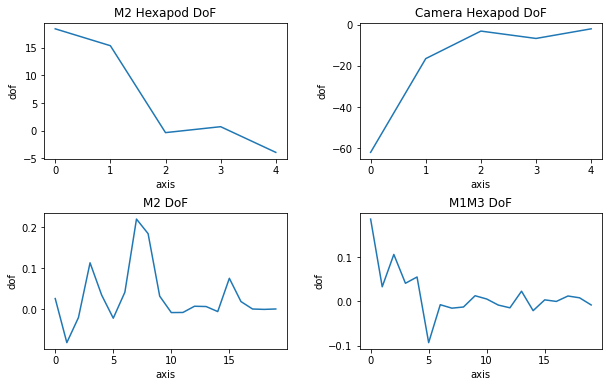
Degrees of Freedom
dof = await mtcs.rem.mtaos.evt_degreeOfFreedom.next(flush=False, timeout=STD_TIMEOUT)
comp_dof_idx = dict(
            m2HexPos=dict(
                startIdx=0,
                idxLength=5,
                state0name="M2Hexapod",
            ),
            camHexPos=dict(
                startIdx=5,
                idxLength=5,
                state0name="cameraHexapod",
            ),
            M1M3Bend=dict(
                startIdx=10, idxLength=20, state0name="M1M3Bending", rot_mat=1.0
            ),
            M2Bend=dict(startIdx=30, idxLength=20, state0name="M2Bending", rot_mat=1.0),
        )
fig, axes = plt.subplots(2,2, figsize=(10,6))

axes[0][0].plot(
    dof.aggregatedDoF[
        comp_dof_idx["m2HexPos"]["startIdx"]:
        comp_dof_idx["m2HexPos"]["startIdx"]+comp_dof_idx["m2HexPos"]["idxLength"]
    ]
)
axes[0][0].set_title("M2 Hexapod DoF")
axes[0][0].set_xlabel("axis")
axes[0][0].set_ylabel("dof")

axes[0][1].plot(
    dof.aggregatedDoF[
        comp_dof_idx["camHexPos"]["startIdx"]:
        comp_dof_idx["camHexPos"]["startIdx"]+comp_dof_idx["camHexPos"]["idxLength"]
    ]
)

axes[0][1].set_title("Camera Hexapod DoF")
axes[0][1].set_xlabel("axis")
axes[0][1].set_ylabel("dof")

axes[1][0].plot(
    dof.aggregatedDoF[
        comp_dof_idx["M2Bend"]["startIdx"]:
        comp_dof_idx["M2Bend"]["startIdx"]+comp_dof_idx["M2Bend"]["idxLength"]
    ]
)
axes[1][0].set_title("M2 DoF")
axes[1][0].set_xlabel("axis")
axes[1][0].set_ylabel("dof")


axes[1][1].plot(
    dof.aggregatedDoF[
        comp_dof_idx["M1M3Bend"]["startIdx"]:
        comp_dof_idx["M1M3Bend"]["startIdx"]+comp_dof_idx["M1M3Bend"]["idxLength"]
    ]
)
axes[1][1].set_title("M1M3 DoF")
axes[1][1].set_xlabel("axis")
axes[1][1].set_ylabel("dof")

fig.patch.set_facecolor('white')
plt.subplots_adjust(hspace=0.4, wspace=0.3)
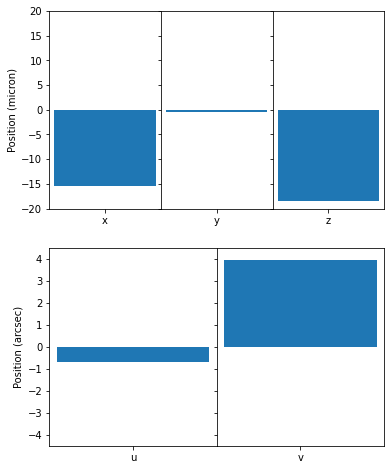
M2 Hexapod Corrections
m2_hex = await mtcs.rem.mtaos.evt_m2HexapodCorrection.next(flush=False, timeout=STD_TIMEOUT)
fig = plt.figure(figsize=(6,8))

axis = []
for panel, label in enumerate("xyz"):

    ax = plt.subplot(2,3,panel+1)

    x = [0.]

    ax.bar(
        [0.0],
        getattr(m2_hex, label),
        width=0.5
    )
    ax.set_xticks([0])
    ax.set_xticklabels([label])
    axis.append(ax)
    ax.set_ylim(-20,20)
    if panel > 0:
        ax.set_yticklabels([])

axis[0].set_ylabel("Position (micron)")

for panel, label in enumerate("uv"):

    ax = plt.subplot(2,2,panel+3)

    x = [0.]

    ax.bar(
        [0.],
        getattr(m2_hex, label)*60.*60.,
        width=0.5
    )

    ax.set_xticks([0])
    ax.set_xticklabels([label])
    axis.append(ax)
    ax.set_ylim(-4.5,4.5)
    if panel > 0:
        ax.set_yticklabels([])

axis[3].set_ylabel("Position (arcsec)")
plt.subplots_adjust(wspace=0.)
fig.patch.set_facecolor('white')
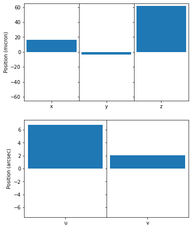
Camera Hexapod Corrections
cam_hex = await mtcs.rem.mtaos.evt_cameraHexapodCorrection.next(flush=False, timeout=STD_TIMEOUT)
fig = plt.figure(figsize=(6,8))

axis = []
for panel, label in enumerate("xyz"):

    ax = plt.subplot(2,3,panel+1)

    x = [0.]

    ax.bar(
        [0.0],
        getattr(cam_hex, label),
        width=0.5
    )
    ax.set_xticks([0])
    ax.set_xticklabels([label])
    if panel > 0:
        ax.set_yticklabels([])
    axis.append(ax)
    ax.set_ylim(-65,65)

axis[0].set_ylabel("Position (micron)")

for panel, label in enumerate("uv"):

    ax = plt.subplot(2,2,panel+3)

    x = [0.]

    ax.bar(
        [0.],
        getattr(cam_hex, label)*60.*60.,
        width=0.5
    )

    ax.set_xticks([0])
    ax.set_xticklabels([label])
    axis.append(ax)
    ax.set_ylim(-7.5,7.5)
    if panel > 0:
        ax.set_yticklabels([])


axis[3].set_ylabel("Position (arcsec)")
plt.subplots_adjust(wspace=0.)

fig.patch.set_facecolor('white')
M1M3 Corrections
m1m3 = await mtcs.rem.mtaos.evt_m1m3Correction.next(flush=False, timeout=STD_TIMEOUT)
m1m3_xact = np.array([ 0.77678278,  1.44256799,  2.10837793,  2.77418799,  3.43999805,
        3.96801294,  0.44386499,  1.10967505,  1.77548499,  2.4412959 ,
        3.10708008,  3.77289111,  0.        ,  0.77678278,  1.44256799,
        2.10837793,  2.77418799,  3.43999805,  3.9005    ,  0.44386499,
        1.10967505,  1.77548499,  2.44127002,  3.10708008,  3.72445288,
        0.        ,  0.77678278,  1.44256799,  2.10837793,  2.77418799,
        3.3879541 ,  0.44386499,  1.10967505,  1.77548499,  2.44127002,
        2.93936401,  0.22194521,  0.88772998,  1.55354004,  2.08973389,
        0.36573459,  1.08508801,  1.60401001, -0.44386499, -1.10968005,
       -1.77548999, -2.44130005, -3.10708008, -3.77288989, -0.77678302,
       -1.44256995, -2.10837988, -2.77418994, -3.44      , -3.9005    ,
       -0.44386499, -1.10968005, -1.77548999, -2.44127002, -3.10708008,
       -3.72444995, -0.77678302, -1.44256995, -2.10837988, -2.77418994,
       -3.38794995, -0.44386499, -1.10968005, -1.77548999, -2.44127002,
       -2.93936011, -0.22194501, -0.88772998, -1.55354004, -2.08972998,
       -0.36573499, -1.08508997, -1.60401001, -0.77678302, -1.44256995,
       -2.10837988, -2.77418994, -3.44      , -3.96801001, -0.44386499,
       -1.10968005, -1.77548999, -2.44130005, -3.10708008, -3.77288989,
        0.        , -0.77678302, -1.44256995, -2.10837988, -2.77418994,
       -3.44      , -3.9005    , -0.44386499, -1.10968005, -1.77548999,
       -2.44127002, -3.10708008, -3.72444995,  0.        , -0.77678302,
       -1.44256995, -2.10837988, -2.77418994, -3.38794995, -0.44386499,
       -1.10968005, -1.77548999, -2.44127002, -2.93936011, -0.22194501,
       -0.88772998, -1.55354004, -2.08972998, -0.36573499, -1.08508997,
       -1.60401001,  0.44386499,  1.10967505,  1.77548499,  2.4412959 ,
        3.10708008,  3.77289111,  0.77678278,  1.44256799,  2.10837793,
        2.77418799,  3.43999805,  3.9005    ,  0.44386499,  1.10967505,
        1.77548499,  2.44127002,  3.10708008,  3.72445288,  0.77678278,
        1.44256799,  2.10837793,  2.77418799,  3.3879541 ,  0.44386499,
        1.10967505,  1.77548499,  2.44127002,  2.93936401,  0.22194521,
        0.88772998,  1.55354004,  2.08973389,  0.36573459,  1.08508801,
        1.60401001])
m1m3_yact = np.array([ 0.        ,  0.        ,  0.        ,  0.        ,  0.        ,
        0.        , -0.57660498, -0.57660498, -0.57660498, -0.57660498,
       -0.57660498, -0.57660498, -1.15320996, -1.15320996, -1.15320996,
       -1.15320996, -1.15320996, -1.15320996, -0.99768701, -1.72981995,
       -1.72981995, -1.72981995, -1.72981995, -1.72981995, -1.51794995,
       -2.30641992, -2.30641992, -2.30641992, -2.30641992, -2.30641992,
       -2.16740991, -2.88303003, -2.88303003, -2.88303003, -2.88303003,
       -2.74517993, -3.45962988, -3.45962988, -3.26742993, -3.43638989,
       -4.00525   , -3.87276001, -3.69278003, -0.57660498, -0.57660498,
       -0.57660498, -0.57660498, -0.57660498, -0.57660498, -1.15320996,
       -1.15320996, -1.15320996, -1.15320996, -1.15320996, -0.99768701,
       -1.72981995, -1.72981995, -1.72981995, -1.72981995, -1.72981995,
       -1.51794995, -2.30641992, -2.30641992, -2.30641992, -2.30641992,
       -2.16740991, -2.88303003, -2.88303003, -2.88303003, -2.88303003,
       -2.74517993, -3.45962988, -3.45962988, -3.26742993, -3.43638989,
       -4.00525   , -3.87276001, -3.69278003,  0.        ,  0.        ,
        0.        ,  0.        ,  0.        ,  0.        ,  0.57660541,
        0.57660541,  0.57660541,  0.57660541,  0.57660541,  0.57660541,
        1.15321106,  1.15321106,  1.15321106,  1.15321106,  1.15321106,
        1.15321106,  0.99768658,  1.72981604,  1.72981604,  1.72981604,
        1.72981604,  1.72981604,  1.51795496,  2.30642212,  2.30642212,
        2.30642212,  2.30642212,  2.30642212,  2.16740698,  2.8830271 ,
        2.8830271 ,  2.8830271 ,  2.8830271 ,  2.74518091,  3.45963208,
        3.45963208,  3.26743091,  3.43639111,  4.00525   ,  3.87276294,
        3.69277905,  0.57660541,  0.57660541,  0.57660541,  0.57660541,
        0.57660541,  0.57660541,  1.15321106,  1.15321106,  1.15321106,
        1.15321106,  1.15321106,  0.99768658,  1.72981604,  1.72981604,
        1.72981604,  1.72981604,  1.72981604,  1.51795496,  2.30642212,
        2.30642212,  2.30642212,  2.30642212,  2.16740698,  2.8830271 ,
        2.8830271 ,  2.8830271 ,  2.8830271 ,  2.74518091,  3.45963208,
        3.45963208,  3.26743091,  3.43639111,  4.00525   ,  3.87276294,
        3.69277905])
fig, axes = plt.subplots(1,1, figsize=(6,6))

img = axes.scatter(
    m1m3_xact,
    m1m3_yact,
    c=m1m3.zForces,
    s=100,
    vmin=-30,
    vmax=30
)

axes.axis('equal')
axes.set_title('M1M3 applied forces')
fig.colorbar(img, ax=axes)
<matplotlib.colorbar.Colorbar at 0x7fcc3c7bb250>

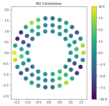
M2 Corrections
m2 = await mtcs.rem.mtaos.evt_m2Correction.next(flush=False, timeout=STD_TIMEOUT)
m2_xact = -np.array([-1.601    , -1.566014 , -1.462585 , -1.295237 , -1.071278 ,
       -0.8005013, -0.4947361, -0.1673502,  0.1673502,  0.4947361,
        0.8005013,  1.071278 ,  1.295237 ,  1.462585 ,  1.566014 ,
        1.601    ,  1.566014 ,  1.462585 ,  1.295237 ,  1.071278 ,
        0.8005013,  0.4947361,  0.1673502, -0.1673502, -0.4947361,
       -0.8005013, -1.071278 , -1.295237 , -1.462585 , -1.566014 ,
       -1.273    , -1.186249 , -1.018657 , -0.7816469, -0.4913655,
       -0.1676011,  0.1675856,  0.4913528,  0.7816342,  1.018647 ,
        1.186244 ,  1.272997 ,  1.273    ,  1.186249 ,  1.018657 ,
        0.7816469,  0.4913655,  0.1676011, -0.1675856, -0.4913528,
       -0.7816342, -1.018647 , -1.186244 , -1.272997 , -1.002    ,
       -0.9415729, -0.7675778, -0.5009998, -0.1739956,  0.1739956,
        0.5009998,  0.7675778,  0.9415729,  1.002    ,  0.9415729,
        0.7675778,  0.5009998,  0.1739956, -0.1739956, -0.5009998,
       -0.7675778, -0.9415729])
m2_yact = -np.array([-1.333500e-16, -3.328670e-01, -6.511849e-01, -9.410446e-01,
       -1.189774e+00, -1.386507e+00, -1.522641e+00, -1.592229e+00,
       -1.592229e+00, -1.522641e+00, -1.386507e+00, -1.189774e+00,
       -9.410446e-01, -6.511849e-01, -3.328670e-01,  0.000000e+00,
        3.328670e-01,  6.511849e-01,  9.410446e-01,  1.189774e+00,
        1.386507e+00,  1.522641e+00,  1.592229e+00,  1.592229e+00,
        1.522641e+00,  1.386507e+00,  1.189774e+00,  9.410446e-01,
        6.511849e-01,  3.328670e-01, -1.675856e-01, -4.913528e-01,
       -7.816342e-01, -1.018647e+00, -1.186244e+00, -1.272997e+00,
       -1.273000e+00, -1.186249e+00, -1.018657e+00, -7.816469e-01,
       -4.913655e-01, -1.676011e-01,  1.675856e-01,  4.913528e-01,
        7.816342e-01,  1.018647e+00,  1.186244e+00,  1.272997e+00,
        1.273000e+00,  1.186249e+00,  1.018657e+00,  7.816469e-01,
        4.913655e-01,  1.676011e-01,  3.893820e-16, -3.427044e-01,
       -6.440729e-01, -8.677580e-01, -9.867773e-01, -9.867773e-01,
       -8.677580e-01, -6.440729e-01, -3.427044e-01,  0.000000e+00,
        3.427044e-01,  6.440729e-01,  8.677580e-01,  9.867773e-01,
        9.867773e-01,  8.677580e-01,  6.440729e-01,  3.427044e-01])
fig, axes = plt.subplots(1,1, figsize=(6,6))

img = axes.scatter(
    m2_xact,
    m2_yact,
    c=m2.zForces,
    s=200,
    vmin=-10.0,
    vmax=10.0
)

axes.axis('equal')

fig.colorbar(img, ax=axes)

fig.patch.set_facecolor('white')
axes.set_title(
    "M2 Corrections",
)
Text(0.5, 1.0, 'M2 Corrections')
Issue correction
After processing is completed we can issue the correction to the AOS components. This will cause the MTAOS to send commands to the M1M3, M2, Camera Hexapod and M2 Hexapod.
If the command fails, make sure all the components above are in enable state. It will also fail if M1M3 is not raised, so make sure you have executed the steps in Setup M1M3.
await mtcs.rem.mtaos.cmd_issueCorrection.start()
<ddsutil.MTAOS_ackcmd_fd03e870 at 0x7fce73e90ca0>
Finalizing
Once the test is complete you may to reset the system to its original state.
This in general mean, reseting the forces on M1M3 and M2, the offsets in the Camera and M2 Hexapods and re-configuring the MTAOS with the original configuration.
Nonte that there is also a step to lower m1m3. If you intend to continue exercicing the system, you may want to sky this step, especially if executing at the summit.
The following cells will execute this procedure, and leave the system in ENABLED state, which is the default for TTS and in general when executing continuous tests at the summit as well.
await mtcs.reset_m1m3_forces()
await mtcs.lower_m1m3()
await mtcs.reset_m2_forces()
await mtcs.reset_camera_hexapod_position()
The following cells will enable compensation mode and reset the position of the M2 Hexapod.
await mtcs.reset_m2_hexapod_position()
To execute IMpf we need to load a special configuration on the MTAOS. This configuration will make sure the MTAOS is reading data from a butler instance that was previously prepared for the test, and will also make sure the MTAOS is configured for processing LSSTCam Corner Wavefront Sensor data.
We start the process by first sending the MTAOS to STANDBY then sending it back to ENABLED with the required configuration.
await mtcs.set_state(
    state=salobj.State.STANDBY,
    components=["mtaos"]
)
await mtcs.set_state(
    state=salobj.State.ENABLED,
    components=["mtaos"]
)