Inspect WEP¶

This notebook is part of the Integration Milestone pf, which involves processing LSSTCam corner wavefront sensor data with the MTAOS and issuing correction to the AOS components.

This notebook is designed to inspect the results of the WEP execution by inspecting the data stored in the butler.

Details about the milestone, execution and verification can be found in tstn-031.

import numpy as np
import os

from lsst.daf import butler as dafButler
import lsst.afw.cameraGeom.utils as cameraGeomUtils
import lsst.afw.display as afwDisplay
import matplotlib.pyplot as plt
from matplotlib import rcParams
from astropy.io import fits
from astropy.visualization import ZScaleInterval

instrument = "LSSTCam"
repo_dir = "/scratch/IM_Pf/LSSTCam"

The DM pipeline run name¶

The following cell specify the wep “run name”. This string is generated by the MTAOS when executing the runWEP command and is used in the butler to differentiate between different executions of the pipeline.

For now, this value is sent by the MTAOS as a log message so, when executing the integration milestone you will have to inspect the logs to find the associated entry. In the future the MTAOS will publish this information as an event, which will make it easier to determine it’s value during the execution.

mtaos_run = "mtaos_wep_tribeiro_nb_tribeiro_20220304T234403714"

butler = dafButler.Butler(
    repo_dir,
    collections=[
        f"{instrument}/raw/all",
        mtaos_run,
    ],
)

exp_num = 4021123110021

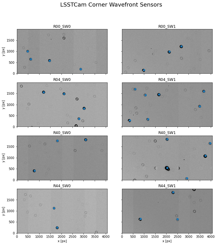
Corner Wavefront Sensors and Source Selection¶

The following is a display of the post-isr corner wavefront sensor data overlaid with the positions of the selected sources.

fig, ax = plt.subplots(4, 2, figsize=(12,12))

for index, detector in enumerate(
    [
    'R00_SW0',
    'R00_SW1',
    'R04_SW0',
    'R04_SW1',
    'R40_SW0',
    'R40_SW1',
    'R44_SW0',
    'R44_SW1'
    ]
):

    post_isr_exposure = butler.get(
        "postISRCCD",
        detector=detector,
        instrument=instrument,
        exposure=exp_num,
        collections=[mtaos_run],
    )

    donut_catalog = butler.get(
        "donutCatalog",
        detector=detector,
        instrument=instrument,
        visit=exp_num,
        collections=[mtaos_run],
    )

    data = post_isr_exposure.image.array

    zscale = ZScaleInterval()

    vmin, vmax = zscale.get_limits(data)

    line = int(np.floor(index / 2))
    column = index % 2


    ax[line][column].imshow(
        post_isr_exposure.image.array,
        vmin=vmin,
        vmax=vmax,
        cmap="Greys",
        origin="lower"
    )

    ax[line][column].scatter(
        donut_catalog["centroid_x"],
        donut_catalog["centroid_y"],
    )

    ax[line][column].set_title(f"{post_isr_exposure.getDetector().getName()}")

    if line == 3:
        ax[line][column].set_xlabel("x [px]")

    if column == 0:
        ax[line][column].set_ylabel("y [px]")

    if column == 1:
        ax[line][column].set_yticklabels([])

    if line < 3:
        ax[line][column].set_xticklabels([])

fig.suptitle(
    f"{instrument} Corner Wavefront Sensors",
    fontsize=18
)
plt.subplots_adjust(wspace=0.)

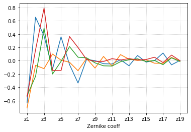
Average Zernike Values¶

The following is a plot of the resulting wavefront errors averaged for each corner wavefront sensor.

fig, ax = plt.subplots(1, 1)

for detector in [191, 195, 199, 203]:
    zernike_estimate_avg = butler.get(
        "zernikeEstimateAvg",
        detector=detector,
        instrument=instrument,
        visit=exp_num,
        collections=[mtaos_run],
    )
    ax.plot(zernike_estimate_avg)

x_ticks = np.arange(0, 19, 2)
ax.set_xticks(x_ticks)
ax.set_xticklabels([f"z{index+1}" for index in x_ticks])
ax.set_xlabel("Zernike coeff")

ax.grid(linestyle=":")

TSTN-031: Integration Milestone Pf

Inspect WEP¶

The DM pipeline run name¶

Corner Wavefront Sensors and Source Selection¶

Average Zernike Values¶